rsgeo is an interface to the Rust libraries geo-types and geo. geo-types implements pure rust geometry primitives. The geo library adds additional algorithm functionalities on top of geo-types. This package lets you harness the speed, safety, and memory efficiency of these libraries. geo-types does not support Z or M dimensions. There is no support for CRS at this moment.
# install.packages(
#   'rsgeo',
#   repos = c('https://josiahparry.r-universe.dev', 'https://cloud.r-project.org')
# )
library(rsgeo)
rsgeo works with vectors of geometries. When we compare this to sf this is always the geometry column which is a class sfc object (simple feature column).
# get geometry from sf
data(guerry, package = "sfdep")

polys <- guerry[["geometry"]] |>
  sf::st_cast("POLYGON")

# cast to rust geo-types
rs_polys <- as_rsgeo(polys)

head(rs_polys)
#> <rs_POLYGON[6]>
#> [1] Polygon { exterior: LineString([Coord { x: 801150.0, y: 2092615.0 }, Coord...
#> [2] Polygon { exterior: LineString([Coord { x: 729326.0, y: 2521619.0 }, Coord...
#> [3] Polygon { exterior: LineString([Coord { x: 710830.0, y: 2137350.0 }, Coord...
#> [4] Polygon { exterior: LineString([Coord { x: 882701.0, y: 1920024.0 }, Coord...
#> [5] Polygon { exterior: LineString([Coord { x: 886504.0, y: 1922890.0 }, Coord...
#> [6] Polygon { exterior: LineString([Coord { x: 747008.0, y: 1925789.0 }, Coord...
Cast geometries to sf
sf::st_as_sfc(rs_polys)
#> Geometry set for 116 features
#> Geometry type: POLYGON
#> Dimension:     XY
#> Bounding box:  xmin: 47680 ymin: 1703258 xmax: 1031401 ymax: 2677441
#> CRS:           NA
#> First 5 geometries:
#> POLYGON ((801150 2092615, 800669 2093190, 80068...
#> POLYGON ((729326 2521619, 729320 2521230, 72928...
#> POLYGON ((710830 2137350, 711746 2136617, 71243...
#> POLYGON ((882701 1920024, 882408 1920733, 88177...
#> POLYGON ((886504 1922890, 885733 1922978, 88547...
Calculate the unsigned area of polygons.
bench::mark(
  rust = unsigned_area(rs_polys),
  sf = sf::st_area(polys),
  check = FALSE
)
#> # A tibble: 2 × 6
#>   expression      min   median `itr/sec` mem_alloc `gc/sec`
#>   <bch:expr> <bch:tm> <bch:tm>     <dbl> <bch:byt>    <dbl>
#> 1 rust         55.6µs  57.65µs    16411.     3.8KB     0
#> 2 sf           1.36ms   1.44ms      649.   786.9KB     8.42
Find centroids
bench::mark(
  centroids(rs_polys),
  sf::st_centroid(polys),
  check = FALSE
)
#> # A tibble: 2 × 6
#>   expression                  min   median `itr/sec` mem_alloc `gc/sec`
#>   <bch:expr>             <bch:tm> <bch:tm>     <dbl> <bch:byt>    <dbl>
#> 1 centroids(rs_polys)    174.95µs    213µs     3720.     3.8KB     9.53
#> 2 sf::st_centroid(polys)   2.43ms    2.6ms      359.   892.9KB     4.70
Extract points coordinates
coords(rs_polys) |>
  head()
#>        x       y line_id polygon_id
#> 1 801150 2092615       1          1
#> 2 800669 2093190       1          1
#> 3 800688 2095430       1          1
#> 4 800780 2095795       1          1
#> 5 800589 2096112       1          1
#> 6 800333 2097190       1          1
Plot the polygons and their centroids
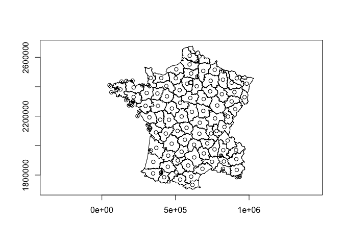
Calculate a distance matrix. Note that there is often floating point error differences so check = FALSE in this case.
pnts <- centroids(rs_polys)
pnts_sf <- sf::st_as_sfc(pnts)

bench::mark(
  rust = distance_euclidean_matrix(pnts, pnts),
  sf = sf::st_distance(pnts_sf, pnts_sf),
  check = FALSE
)
#> # A tibble: 2 × 6
#>   expression      min   median `itr/sec` mem_alloc `gc/sec`
#>   <bch:expr> <bch:tm> <bch:tm>     <dbl> <bch:byt>    <dbl>
#> 1 rust       323.53µs 573.06µs     1540.     108KB     4.08
#> 2 sf           3.48ms   3.69ms      256.     351KB     0
Simplify geometries.
x <- rs_polys
x_simple <- simplify_geoms(x, 5000)

plot(x_simple)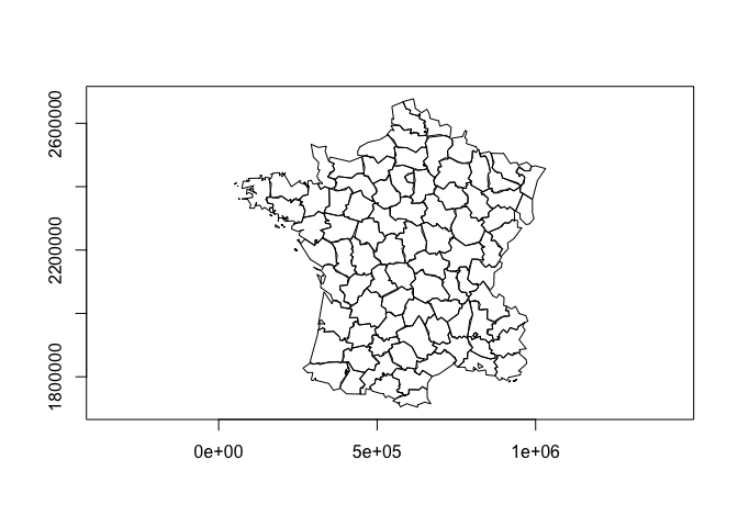
bench::mark(
  rust = simplify_geoms(rs_polys, 500),
  sf = sf::st_simplify(polys, FALSE, 500),
  check = FALSE
)
#> # A tibble: 2 × 6
#>   expression      min   median `itr/sec` mem_alloc `gc/sec`
#>   <bch:expr> <bch:tm> <bch:tm>     <dbl> <bch:byt>    <dbl>
#> 1 rust         6.29ms   6.76ms      141.    1.91KB     0
#> 2 sf           8.52ms   9.02ms      108.    1.24MB     2.08
Union geometries with union_geoms(). Some things sf is better at! One of which is performing unary unions of complex geometries.
plot(union_geoms(rs_polys))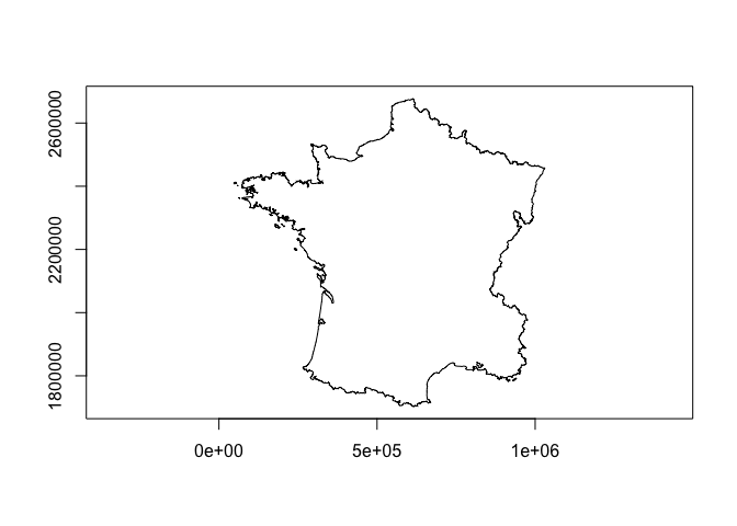
bench::mark(
  union_geoms(rs_polys),
  sf::st_union(polys),
  check = FALSE
)
#> # A tibble: 2 × 6
#>   expression                 min   median `itr/sec` mem_alloc `gc/sec`
#>   <bch:expr>            <bch:tm> <bch:tm>     <dbl> <bch:byt>    <dbl>
#> 1 union_geoms(rs_polys)    205ms    209ms      4.78        0B        0
#> 2 sf::st_union(polys)      120ms    134ms      7.49     921KB        0
We can cast between geometries as well.
lns <- cast_geoms(rs_polys, "linestring")Some unions are faster when using rsgeo vectors like linestrings.
lns_sf <- sf::st_cast(polys, "LINESTRING")

bench::mark(
  union_geoms(lns),
  sf::st_union(lns_sf),
  check = FALSE
)
#> # A tibble: 2 × 6
#>   expression                min   median `itr/sec` mem_alloc `gc/sec`
#>   <bch:expr>           <bch:tm> <bch:tm>     <dbl> <bch:byt>    <dbl>
#> 1 union_geoms(lns)      117.5µs    174µs    4275.         0B     0
#> 2 sf::st_union(lns_sf)   87.8ms     94ms      10.7    2.46MB     2.68
Find the closest point to a geometry
close_pnt <- closest_point(
  rs_polys,
  geom_point(800000, 2090000)
)

plot(rs_polys[1])
plot(close_pnt, pch = 15, add = TRUE)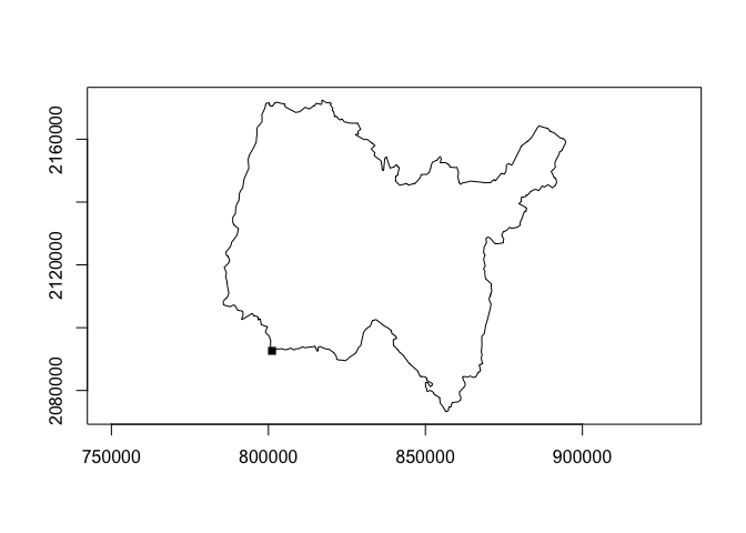
Find the haversine destination of a point, bearing, and distance. Compare to the very fast geosphere destination point function.
bench::mark(
  rust = haversine_destination(geom_point(10, 10), 45, 10000),
  Cpp = geosphere::destPoint(c(10, 10), 45, 10000),
  check = FALSE
)
#> # A tibble: 2 × 6
#>   expression      min   median `itr/sec` mem_alloc `gc/sec`
#>   <bch:expr> <bch:tm> <bch:tm>     <dbl> <bch:byt>    <dbl>
#> 1 rust         5.86µs   7.34µs   120442.     3.2KB     12.0
#> 2 Cpp         17.06µs  19.11µs    34150.    11.8MB     34.2
origin <- geom_point(10, 10)
destination <- haversine_destination(origin, 45, 10000)
plot(c(origin, destination), col = c("red", "blue"))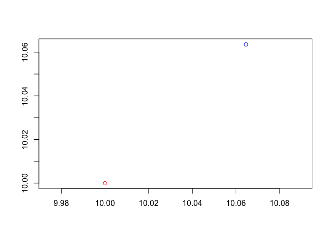
Find intermediate point on a great circle.
middle <- haversine_intermediate(origin, destination, 1/2)

plot(origin)
plot(destination, add = TRUE, col = "red")
plot(middle, add = TRUE, col = "blue")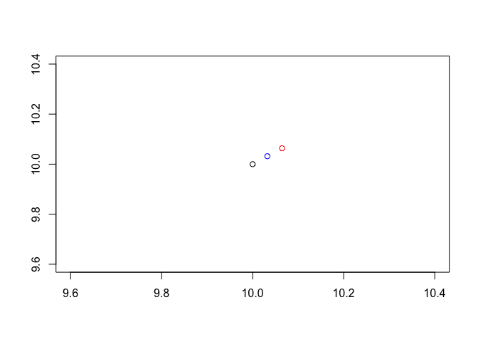
Find extreme coordinates with extreme_coords()
france <- union_geoms(rs_polys)

plot(france)
plot(extreme_coords(france)[[1]], add = TRUE, pch = 15)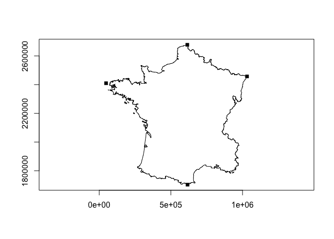
Get bounding rectangles
rects <- bounding_rect(rs_polys)
plot(rects)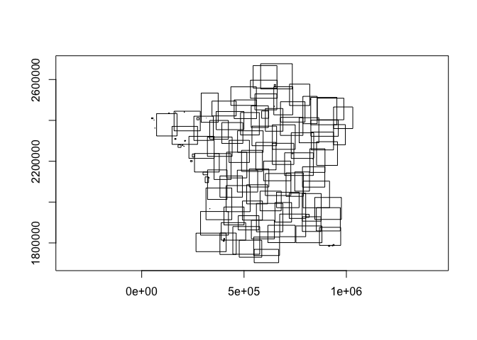
Convex hulls
convex_hull(rs_polys) |>
  plot()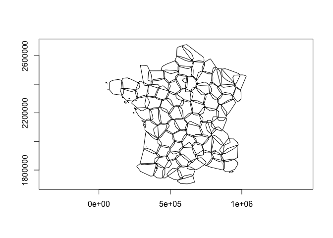
Expand into constituent geometries as a list of geometry vectors
expand_geoms(rs_polys) |>
  head()
#> [[1]]
#> <rs_LINESTRING[1]>
#> [1] LineString([Coord { x: 801150.0, y: 2092615.0 }, Coord { x: 800669.0, y: 2...
#>
#> [[2]]
#> <rs_LINESTRING[2]>
#> [1] LineString([Coord { x: 729326.0, y: 2521619.0 }, Coord { x: 729320.0, y: 2...
#> [2] LineString([Coord { x: 647667.0, y: 2468296.0 }, Coord { x: 647777.0, y: 2...
#>
#> [[3]]
#> <rs_LINESTRING[1]>
#> [1] LineString([Coord { x: 710830.0, y: 2137350.0 }, Coord { x: 711746.0, y: 2...
#>
#> [[4]]
#> <rs_LINESTRING[1]>
#> [1] LineString([Coord { x: 882701.0, y: 1920024.0 }, Coord { x: 882408.0, y: 1...
#>
#> [[5]]
#> <rs_LINESTRING[1]>
#> [1] LineString([Coord { x: 886504.0, y: 1922890.0 }, Coord { x: 885733.0, y: 1...
#>
#> [[6]]
#> <rs_LINESTRING[1]>
#> [1] LineString([Coord { x: 747008.0, y: 1925789.0 }, Coord { x: 746630.0, y: 1...
We can flatten the resultant geometries into a single vector using flatten_geoms()
expand_geoms(rs_polys) |>
  flatten_geoms() |>
  head()
#> <rs_LINESTRING[6]>
#> [1] LineString([Coord { x: 801150.0, y: 2092615.0 }, Coord { x: 800669.0, y: 2...
#> [2] LineString([Coord { x: 729326.0, y: 2521619.0 }, Coord { x: 729320.0, y: 2...
#> [3] LineString([Coord { x: 647667.0, y: 2468296.0 }, Coord { x: 647777.0, y: 2...
#> [4] LineString([Coord { x: 710830.0, y: 2137350.0 }, Coord { x: 711746.0, y: 2...
#> [5] LineString([Coord { x: 882701.0, y: 1920024.0 }, Coord { x: 882408.0, y: 1...
#> [6] LineString([Coord { x: 886504.0, y: 1922890.0 }, Coord { x: 885733.0, y: 1...
Combine geometries into a single multi- geometry
combine_geoms(lns)
#> <rs_LINESTRING[1]>
#> [1] MultiLineString([LineString([Coord { x: 801150.0, y: 2092615.0 }, Coord { ...
Spatial predicates
x <- rs_polys[1:5]
intersects_sparse(x, rs_polys)
#> [[1]]
#> [1]  1 48 50 92 94
#>
#> [[2]]
#> [1]   2   7  63  78  80  81  98 101
#>
#> [[3]]
#> [1]  3 20 27 53 77 84 94
#>
#> [[4]]
#> [1]   4   5  30 107 109
#>
#> [[5]]
#> [1]  4  5 30 48